Probabilities of Up and Down Days in the S&P500

[Last Updated: 11/24/2024]

In this post we’ll be calculating the probabilities and statistics of up days and down days.

First, I’ll use daily S&P 500 (Ticker: SPY) data to obtain probabilities of up and down days. Next, we’re going to look at various other related topics such as:

1. Determining the probabilities of consecutive up and down days
2. Extending the timeframe of the data from daily candlesticks to weekly candlesticks
3. Applying the same statistical analysis to each sector ($XLY, $XLK, etc.) instead of just the $SPY

The Probability of Up and Down Days in the S&P 500

The data we’re going to use is recent market data starting from January 2020 and ending in November 2024, the time this blog post is being written. To obtain market data we’re going to use the yfinance Python library.

Importing SPY Data

First, import your modules:

import pandas as pd # Used later
import yfinance as yf
import matplotlib.pyplot as plt # Used later
from math import factorial as fac # Used later

Next, import the historical S&P 500 data from 1/1/2020 to 11/20/2024:

# Obtain historical SPY data
SPY = yf.Ticker("SPY")
start = "2020-01-01"
end = "2024-11-20"
interval = "1d"

df_ticker = SPY.history(period="max", interval=interval, start=start, end=end , auto_adjust=True, rounding=True)
df = df_ticker[["Open", "Close"]]

You can chose to import other dates of course, but you will receive different results.

Computing the Up/Down/No Change Columns

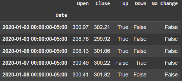
Next, we need a way to label the direction of each row. I decided to add columns (Up, Down, and No Change) which hold boolean values indicating whether the day is an up day, a down day, or a no-change day.

For example, if the Open/Close data in a given row indicate that the direction for that day is an UP day, then the value in the Up column will be TRUE while the values in the Down and No Change columns will be FALSE.

df["Up"] = df["Open"] < df["Close"]
df["Down"] = df["Open"] > df["Close"]
df["No Change"] = df["Open"] == df["Close"]

Figure 1 shows a preview of the data contained in the dataframe after creating the Up/Down/No Change columns.

Calculating the Number of Up and Down Days

To calculate the number of Up and Down days, use the sum function on the related column in the dataframe. The (axis=0) argument of the sum function tells pandas we want to count the number of TRUE values down the column.

up_days = df["Up"].sum(axis=0)
down_days = df["Down"].sum(axis=0)
no_change_days = df["No Change"].sum(axis=0)
number_of_observations = df.shape[0]

up_days, down_days, no_change_days, number_of_observations

>> (676, 552, 2, 1230)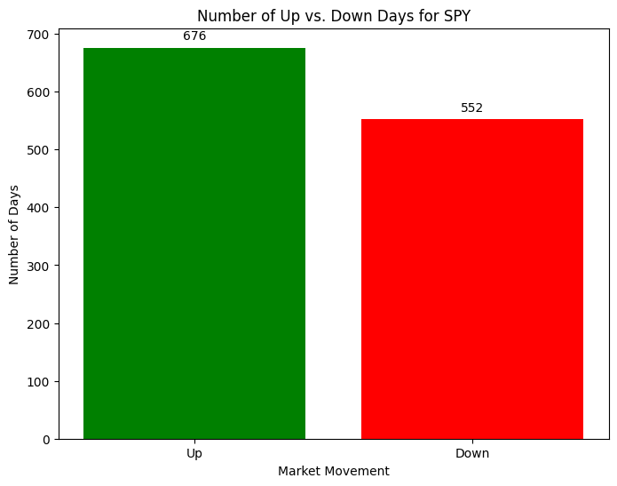

Up Day vs. Down Day Ratios in the S&P500

The ratio of Up days in the S&P 500 between January 2020 and November 2024 was 676 / 1230 = 0.5496, or 54.96%.

# Probability of an UP day:
probability_of_up = up_days / number_of_observations

>> 0.5495934959349593

And the ratio of Down days in the S&P 500 between the same time frame is 552 / 1230 = 0.44878, or 44.878%.

# Probability of a DOWN day:
probability_of_down = down_days / number_of_observations

>> 0.44878048780487806

Probability of Consecutive Days

If we take these ratios as probabilities for future outcomes, then we can model the S&P500 as a series of Bernoulli trials with probability p = 54.959%.

The probability of consecutively occurring “up” days is given by the B(n,p,k) in Equation 1:

Since we’re looking for consecutive up days, we set n = k. That means the binomial coefficient is equal to 1, the exponential (n – k) is equal to 0, and q^0 = 1. The only term that matters in our case is p^k.

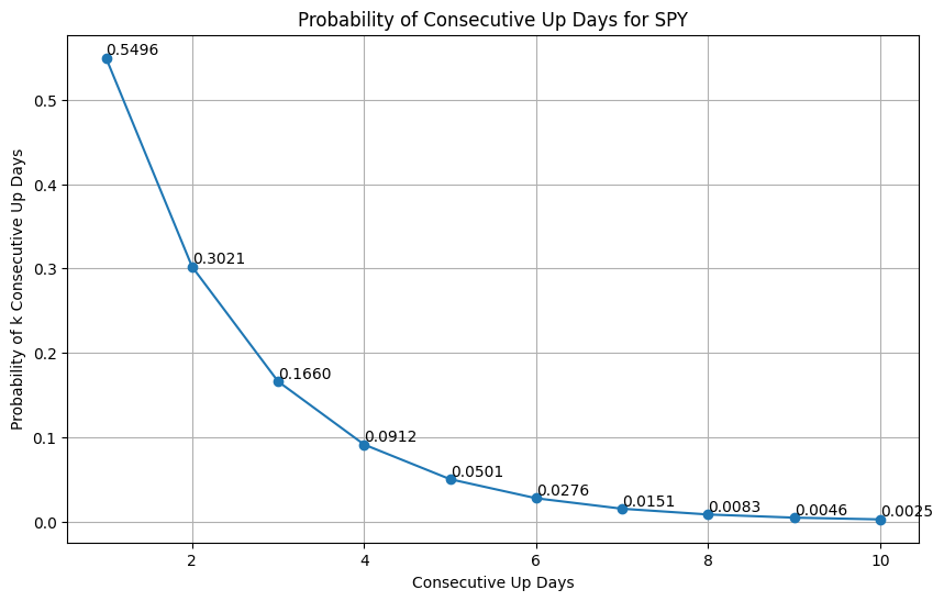
We can calculate and visualize the probability of consecutive up days from 1 to 10 days with a line plot (Figure 3). It becomes substantially unlikely to see over 2 or 3 consecutive up days. Two consecutive up days are expected 30.21% of the time, while three consecutive up are expected 16.6% of the time.

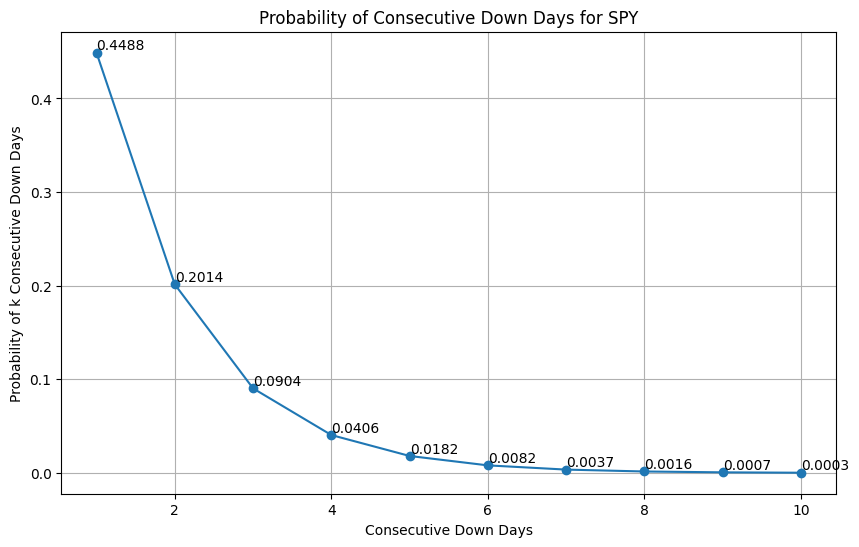
The same thing can be done for consecutive down days, just with the starting probability changed to 0.4488.

Two Contra-Directional Days

One might ask what the probability is of a “switch-a-roo” situation where the market flips from one candlestick direction to the other. For this, we’ll take the up and down ratios we calculated above and use them to calculate the probability of an Up-Then-Down situation and a Down-Then-Up situation. This assumes a Bernoulli process where each day has probabilities of success that are independent and identical.

Predictions Using Bernoulli Trials

The probability of an Up day was calculated to be 0.5496. For a down day, 0.4488. If we’re modeling the market as a process of independently and identically occuring events, then we can estimate that these probabilities hold for each and every day.

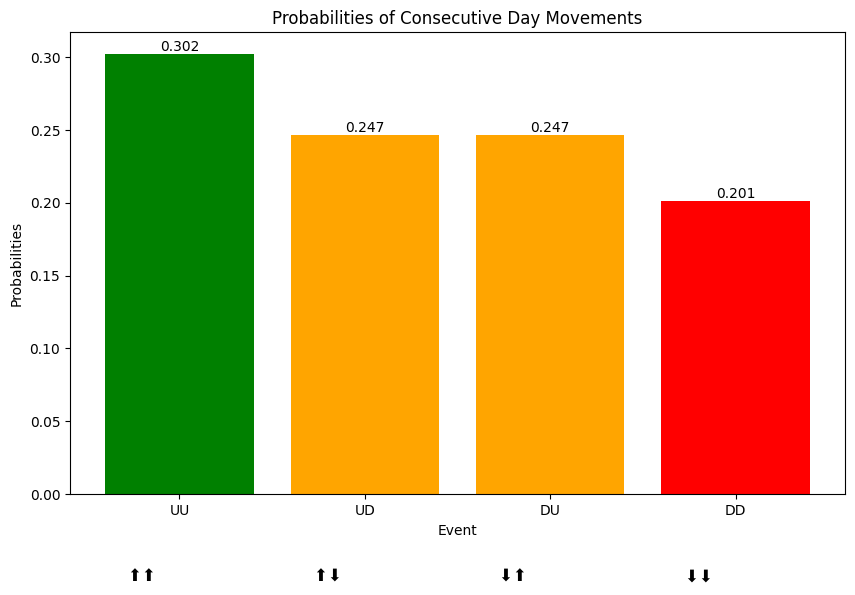
The probability of an “up-then-down” day is p * q = 0.5496 * 0.4488 = 0.24665 = 24.67%. The probability of a “down-then-up” day is exactly the same (q * p).

Figure 5, below, breaks down the two-day sequential probabilities calculated here and in the prior section. As a reminder, the probability of two consecutive up days was ~30.2%, while the probability of two consecutive down days was ~20.1%.

Testing the Predictions Against the Sample Statistics

While the above calculations for the switch-a-roo events are based on actual data, they are not the actual statistics themselves. Let’s see how correct it is to assume a Bernoulli model for this data by analyzing the data.

The code for counting these events is below. We iterate through every row of the dataframe, excluding the first row, and count all the instances of two-day sequences (UU, UD, DU, DD):

up_then_down_count = 0
down_then_up_count = 0
for i in range(1, len(df)):
    if df["Up"][i-1] and df["Down"][i]:
        up_then_down_count += 1
      
    if df["Down"][i-1] and df["Up"][i]:
        down_then_up_count += 1
    
    if df["Down"][i-1] and df["Down"][i]:
        down_then_down_count += 1
      
    if df["Up"][i-1] and df["Up"][i]:
        up_then_up_count += 1

up_then_up_count, up_then_down_count, down_then_up_count, down_then_down_count, len(df)-1

>> (359, 315, 314, 237,1229)

The probabilities are computed as:

• Up-then-up: 0.2921 = 29.21%
• Up-then-down: 0.2563 = 25.63%
• Down-then-up: 0.2555 = 25.55%
• Down-then-down: 0.1928 = 19.28%

These probabilities are just about in line (within +/- 1%) with the modeled counts above, making the model relatively accurate for this time frame. Those who are savvy might realize that the percentages above add up to only 99.67%. That’s because some of the days may start and end at the same price, which aren’t included in the counts above. Since these days account for less than 0.5% in this case, I feel comfortable leaving these out of the calculations.

One might ask, given an up day, what is the probability that the next day is also an up day? For that, we calculate the probability of two consecutive up days (0.292) and divide it by the probability that an up day occurred on the first day (0.292 + 0.256). The result is 0.533 = 53.3%. This is slightly lower to the initial probability that any day is an up day (54.96%).

Additionally, you might ask about the probability that the market reverts upwards after a down day. Calculate the probability of a down-then-up day (0.255) and divide it by the probability that a down day occurred on the first day (0.255 + 0.193). The result is 0.569 = 56.9%.

So, during the period between 2020 and 2024, it was more likely that the market would increase if a down day was experienced first (56.9% for a down-then-up day > 53.3% for an up-then-up day). Therefore, buy-the-dippers saw a slight advantage between 2020 and 2024.

Now, let’s consider weekly data:

Probability of Up & Down Weeks

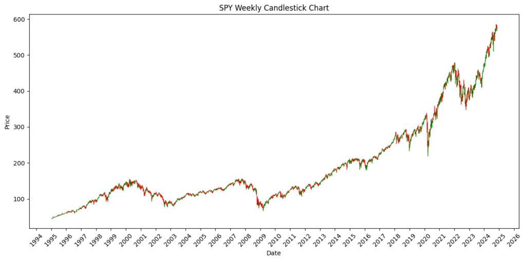
Let’s broaden our scope to weekly data. We’ll look at weekly SPY prices from January 1995 to November 2nd, 2024. To do that, we first need to download the daily pricing data using yfinance:

df = yf.download("SPY", group_by="ticker", start="1995-01-01", end="2024-11-02")
df_daily_close = df["SPY"].loc[:, ["Close", "Open", "High", "Low"]]
df_daily_close.head()

Then we need to convert that daily data into weekly data through aggregation and resampling:

functions = {"Open": "first", "High": "max", "Low": "min", "Close": "last"}
df_weekly_ohlc = df_daily_close.resample('W-FRI').aggregate(functions)
df_weekly_ohlc.head()

Plotting a candlestick chart of the weekly SPY data should yield the following plot:

Now that we have the weekly data we can apply the same conditional categorization on the OHLC data using the following:

df_weekly_ohlc["Up"] = df_weekly_ohlc["Open"] < df_weekly_ohlc["Close"]
df_weekly_ohlc["Down"] = df_weekly_ohlc["Open"] > df_weekly_ohlc["Close"]
df_weekly_ohlc["No Change"] = df_weekly_ohlc["Open"] == df_weekly_ohlc["Close"]
df_weekly_ohlc.head()

Calculating the total number of up and down weeks, along with their ratios, is straightforward:

# Number of up and down weeks
up_weeks = df_weekly_ohlc["Up"].sum(axis=0)
down_weeks = df_weekly_ohlc["Down"].sum(axis=0)
no_change_weeks = df_weekly_ohlc["No Change"].sum(axis=0)

# Probability of up and down weeks
probability_of_up = up_weeks / number_of_weeks
probability_of_down = down_weeks / number_of_weeks
probability_of_no_change = no_change_weeks / number_of_weeks

probability_of_up, probability_of_down
>> (0.5497752087347463, 0.4482980089916506)

As you can see, the ratios up weeks and down weeks from 1995 to 2024 is roughly the same as the daily probabilities within the last four years from 2020 to 2024. Thus, it can be postulated that there is not much statistical difference between investing on a weekly basis vs. a daily basis (at least for the timeframes I’ve sampled from in this article). Further work should be done to clarify that postulation.

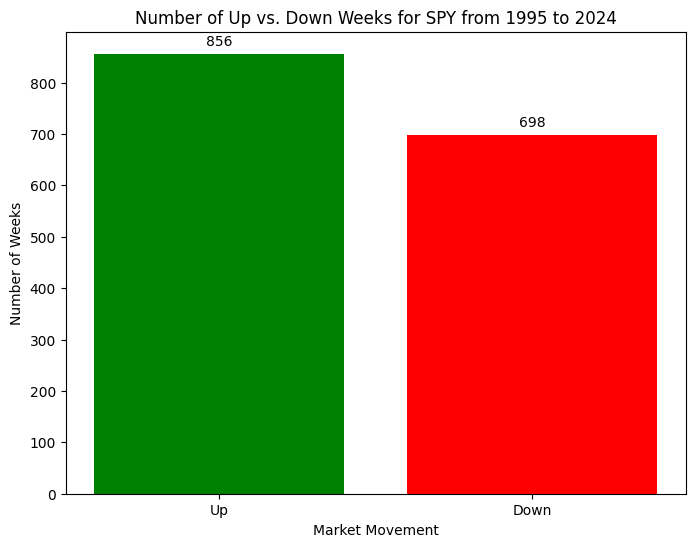
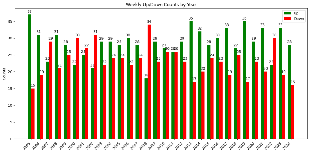
Out of completeness I generated the following figures. Figure 7 below shows the total number of up vs. down weeks in the SPY from 1995 to 2024. Figure 8 shows the same results on a per year basis.

Diving into the S&P500 Sectors

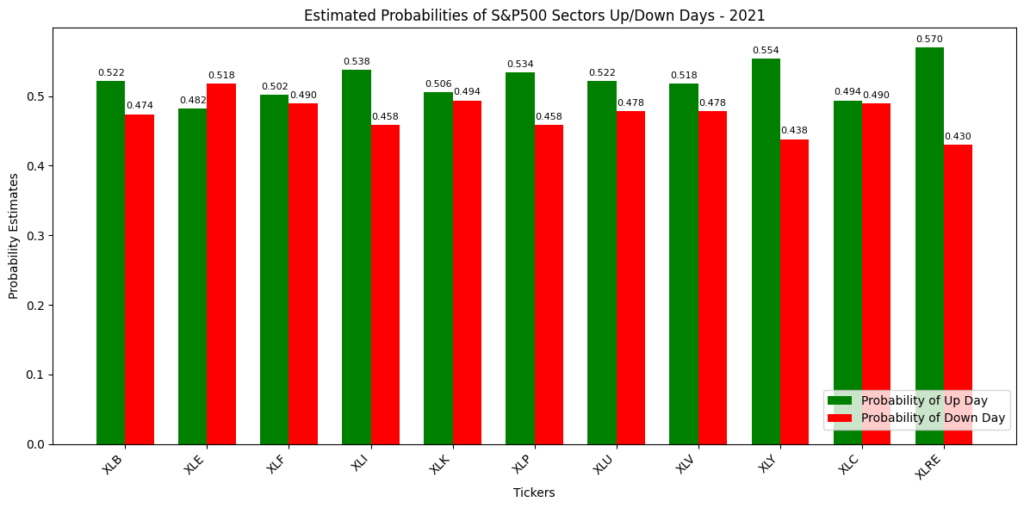
Next we’re going to look at up vs. down directional data for each of the 11 S&P500 Sector ETFs. We’re going to focus on two years: 2021 and 2022.

In 2021, the number of up and down days for each sector can be expressed as a grouped bar chart, with one group per sector ETF.

The same chart can be constructed for 2022 data:

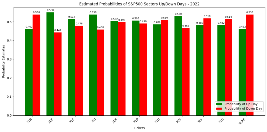
As can be seen, just by looking at the number of up and down days, there is clear evidence that S&P500 sectors behaved much differently. For example, in 2021 the real estate sector (XLRE) had a larger percentage of up days (57%), while in 2022 that ratio fell to 46.2%. These statistics could be used as outcomes of larger macro or microeconomic phenomena.

For example, the higher XLRE up-day ratio in 2021 could be indicative of a COVID-19 comeback rally due to many factors: vaccine availability, higher value in home-ownership (more isolation), and historically low interest rates. Conversely, the lower ratio in 2022 could be explained by the initial shock of the Federal Reserve initiating rate hikes to curb inflation.