Using a Random Forest Classifier to Classify Candlesticks

[Last Updated: 4/20/2025]

Going through my current Data Science & Analytics studies, I was interested in applying a basic supervised learning model to kick off my understanding of Machine Learning applications. I decided to focus on using a random forest classifier to classify candlesticks.

Candlesticks are visual abstractions of pricing patterns in the stock market for a given period of time (ex. 1 day). They hold information about the starting price (Open), the closing price (Close), the highest price (High) and the lowest price (Low) during a given period of time.

In this article, I show how I used Python and mplfinance to manually label the candlestick data and how I trained a Random Forest Classifier to classify new observations of candlesticks.

For the code related to this article, visit the GitHub repo here.

Choosing a Manual Labeling Scheme

To manually label data you need an idea of the features you’re going to use to differentiate the classes. I built this visual guide to help me manually label each candlestick.

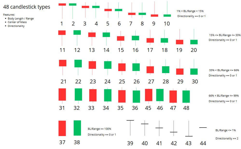
There was some feature engineering that had to be done, since OHLC pricing data varies widely between each ticker. Because of this, I tried to choose features that were relative values (%) versus absolute ($).

There are five (5) main features that I used to manually classify candlesticks:

• Body to Range Ratio
• Center of Mass (more here)
• Direction
• Upper Wick Length to Range Ratio
• Lower Wick Length to Range Ratio

The following code gives you an idea of how I calculated each of these features.

# Compute Range = High - Low
df['Range'] = df['High'] - df['Low']

# Compute Body Length = abs(Close - Open)
df['Body'] = abs(df['Close'] - df['Open'])

# Compute proportion of body length to range
df['BodyRangeRatio'] = df['Body'] / df['Range']

# Compute the direction of candle
threshold = 0.001
df['Direction'] = df.apply(
    lambda row: 2 if abs(row['Open'] - row['Close']) < threshold else (1 if row['Close'] > row['Open'] else 0),
    axis=1
)  # 2 = Doji, 1 = Bullish, 0 = Bearish

# Computer the center of mass (location of the body center in relation to the range)
df['CoM'] = (df[['Open', 'Close']].mean(axis=1) - df['Low']) / df['Range'] 

# Compute Proportion of candle upper wick to range
df['UpperWick'] = (df['High'] - df[['Open', 'Close']].max(axis=1)) / df['Range']

# Compute Proportion of candle lower wick to range
df['LowerWick'] = (df[['Open', 'Close']].min(axis=1) - df['Low']) / df['Range']

Labeling Candlesticks

Since I used quantifiable values to differentiate each candlestick, it was quite difficult to perform manual labeling just by looking at the numbers. I had to develop a program that helped with this, which you can find in the file labeled step01-labeling.py.

The steps are as follows:

1. Import daily OHLC data from yfinance.
2. Calculate relevant features.
3. Select the number of rows you want to label.
4. Run the program and start the labeling process by:
   • Visualizing the candlestick and calculated features for quick identification.
   • Label the candlestick.
5. Repeat #4 until all N rows are labeled.
6. Generate a CSV file with the labeled data.

Below is a run through of the code that helped with this process. It depends on the following imports:

from datetime import datetime
import yfinance as yf
import pandas as pd
import mplfinance as mpf
import matplotlib.pyplot as plt

Importing Daily OHLC Data

ticker = "KO"
today = datetime.now().strftime('%Y-%m-%d')
data = yf.Ticker(ticker).history(start="2007-01-01", end=today)
df = data[["Open", "High", "Low", "Close"]].copy()

Calculate Relevant Features

See the feature engineering code above.

Select Number of Rows to Label

Use the variable N to select the number of rows you wish to label.

# Select just the first N rows to manually label
N = 250
training_df = df.head(N).copy()

Run and Label the Candlesticks

The code for this section runs a for loop that pulls out a single candlestick from the dataset, displays it for visualization, and adds labels holding the calculated features.

After visualizing the plot, you can easily classify the candlestick using the classification paradigm and assign the corresponding label to that observation. This repeats N times until all rows are labeled.

Here is an example of what appears during each iteration:

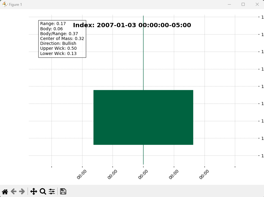
Once you close the matplotlib window, an input() command prompts you to label the candlestick you just saw:

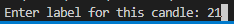
After entering the label and pressing Enter, you can either press Enter again to move onto the next candlestick, or type the letter ‘q’ and press Enter to quit.

Here’s the code:

# Loop through each row in the training dataframe
for idx, row in training_df.iterrows():
    single_candle = pd.DataFrame({
        'Open': [row['Open']],
        'High': [row['High']],
        'Low': [row['Low']],
        'Close': [row['Close']]
    }, index=[pd.to_datetime(row.name)])  # Use index for mplfinance

    # Generate the stat text
    direction_label = (
        'Bullish' if row['Direction'] == 1 else
        'Bearish' if row['Direction'] == 0 else
        'Doji'
    )
    stats_text = (
        f"Range: {row['Range']:.2f}\n"
        f"Body: {row['Body']:.2f}\n"
        f"Body/Range: {row['BodyRangeRatio']:.2f}\n"
        f"Center of Mass: {row['CoM']:.2f}\n"
        f"Direction: {direction_label}\n"
        f"Upper Wick: {row['UpperWick']:.2f}\n"
        f"Lower Wick: {row['LowerWick']:.2f}"
    )

    # Create the plot
    fig, axlist = mpf.plot(
        single_candle,
        type='candle',
        style='charles',
        returnfig=True,
        figratio=(6, 4),
        title=f"Index: {idx}",
        tight_layout=True
    )

    # Annotate stats on the figure
    axlist[0].text(0.05, 0.95, stats_text, transform=axlist[0].transAxes,
                   fontsize=10, verticalalignment='top', bbox=dict(facecolor='white', alpha=0.7))

    # Show and wait for input to move on
    plt.show()

    # Label the candlestick based on your own categorization paradigm
    training_df.loc[idx, 'Label'] = input("Enter label for this candle: ")

    # Save the labeled training data as a CSV
    training_df.to_csv(f"{ticker}-training.csv")

    # Optional: Allow break to stop early
    cont = input("Press [Enter] to continue, or type 'q' to quit: ")
    if cont.lower() == 'q':
        break

Generate a CSV of Labeled Candlestick Data

This step is carried out dynamically in the for loop above using the following line:

training_df.to_csv(f"{ticker}-training.csv")

This ensures that the labels aren’t lost in the event that something goes wrong during the labeling process.

Training the Random Forest Classifier

The idea here is to feed the labeled data to a Random Forest Classifier (from scikit-learn), then use it to label (or “predict”) any new observations based on the training data. The related code for training the classifier is located in step02-training.py.

Here are the dependencies for this file:

import pandas as pd
import matplotlib.pyplot as plt

from sklearn.preprocessing import LabelEncoder
from sklearn.model_selection import train_test_split
from sklearn.ensemble import RandomForestClassifier
from sklearn.metrics import classification_report
import joblib

The steps are as follows:

1. Pull in the training data (X).
2. Define and encode the labeled vector (y).
3. Split the labeled data into train and test sets.
4. Fit the Random Forest Classifier model.
5. Evaluate the model.
6. Save the model.

Pull in Training Data

In our case, the training data is saved in a CSV as KO-training.csv. Pull that in and define the features you want the model to pay attention to. In our case, they are the same five features specified above.

# Define the ticker
ticker = "KO"

# Pull training data from CSV
train_df = pd.read_csv(f"{ticker}-training.csv")

# Define features to include in the training set
features = [
    'BodyRangeRatio',
    'CoM',
    'Direction',
    'UpperWick',
    'LowerWick'
]

# Training Data Set
X = train_df[features]

Define and Encode the Label Vector

The manual labels are saved under the “Label” column in the train_df dataframe. We need to extract that column and encode the labels as unique classes for the model to understand.

# Labeled vector
y = train_df['Label']

# Encode training labels
encoder = LabelEncoder()
y_encoded = encoder.fit_transform(y)

Split into Train and Test Sets

Next, in order to evaluate our model, we need to split the data into training and test sets.

# Split X into testing and training data
X_train, X_test, y_train, y_test = train_test_split(X, y_encoded, test_size=0.1, random_state=42)

Fit the Random Forest Classifier Model

Now it’s time to fit the model to our test data. We do this by instantiating the classifier model with default parameters (n_estimators = 100 and random_state = 42) and calling the fit method using the training data (X_train and y_train).

# Create and fit the Random Forest Classifier model
model = RandomForestClassifier(n_estimators=100, random_state=42)
model.fit(X_train, y_train)

Evaluate the Model

There are two methods I added to evaluate the model:

1. Classification Report
2. Feature Importances

The classification report gives us basic values on model performance, including Precision, Recall, and F1-Score. The feature importances gives us a plot showing the relative “importance” of each feature within the model.

# Compute metrics and classification report, including F1 Score, Precision, and Recall rates
y_pred = model.predict(X_test)
target_names = [str(cls) for cls in encoder.classes_]
print(classification_report(y_test, y_pred, labels=range(len(encoder.classes_)), target_names=target_names))

# Visualize the feature importances
importances = model.feature_importances_
plt.barh(features, importances)
plt.title("Feature Importances")
plt.show()

Save the Model

Now that we’ve trained a model, and the model is giving satisfactory results, we may want to use the model without having to train it every time we want to use it. We can save a snapshot of the trained Random Forest Classifier as a .pkl file using the joblib package.

# Save model as pickle file to upload in other contexts
def save_model(model, encoder, filename):
    joblib.dump(model, filename + '_model.pkl')
    # joblib.dump(encoder, filename + '_encoder.pkl')

save_model(model, encoder, "candlestick_classifier")

Loading the Model

If you wish to use the candlestick_classifier.pkl in the future, you can use the following code to load and utilize the model:

model = joblib.load("candlestick_model.pkl")